Word Cloud of jobs in Data Science

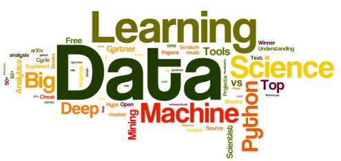
Last updated on Jul 4, 2020 3 min read NLP

Word cloud is a text mining technique to visualize words that give greater prominence to the word appearing more frequently.

In the following sections, we will build word clouds of data science job description in few steps using R. Let’s get started.

1. Create a text data

The data set contains a text of 50 job descriptions(data scientist, data analyst and data engineer) from three US cities - San Francisco, Seattle and New York.

2. Load packages

pacman::p_load(tm,wordcloud,wordcloud2, RColorBrewer)

Note: p_load() function of pacman package loads other packages in R without needing to download them. tm is for text mining - corpus, text cleaning and document term matrix. wordcloud is to generate word cloud and RColorBrewer is for color palettes.

3. Load text data

data_science <- readLines("ds.txt")
data_science <- gsub("[^A-Z  a-z]", "", data_science) # keep characters only

4. Text cleaning

First, load data as a corpus. Corpus contains a list of document. In this case, we have one document.

data_corpus <- Corpus(VectorSource(data_science))

Secondly, we remove words that don’t add context i.e. stop words including some words that are irrelevant in our analysis. Additionally, we utilize other text cleaning techniques.

data_clean <- tm_map(data_corpus,removePunctuation)
data_clean <- tm_map(data_clean,removeWords, c(stopwords("en"), "you",
"data","will","science", "etc", "andor", "including", "experience"))
data_clean <- tm_map(data_clean, stripWhitespace)
data_clean <- tm_map(data_clean, tolower)

5. Document Term Matrix

Our data is in unstructured form. To do further analysis, we convert data to tabular format. This can be achieved via a document term matrix(dtm) which displays a word with its frequency in matrix format.

dtm_data <- TermDocumentMatrix(data_clean)
m <- as.matrix(dtm_data) # convert to matrix
v <- sort(rowSums(m), decreasing = TRUE)
df <- data.frame(word = names(v), frequency = v)
head(df,10) # top 10 words

##                    word frequency
## experience   experience        84
## learning       learning        68
## business       business        67
## models           models        61
## you                 you        57
## machine         machine        56
## work               work        53
## strong           strong        53
## engineering engineering        51
## ability         ability        51

Let’s visualize with bar plot.

w <- rowSums(m)
w <- subset(w, w>=17)
barplot(w,
        las = 2,
        col = rainbow(25))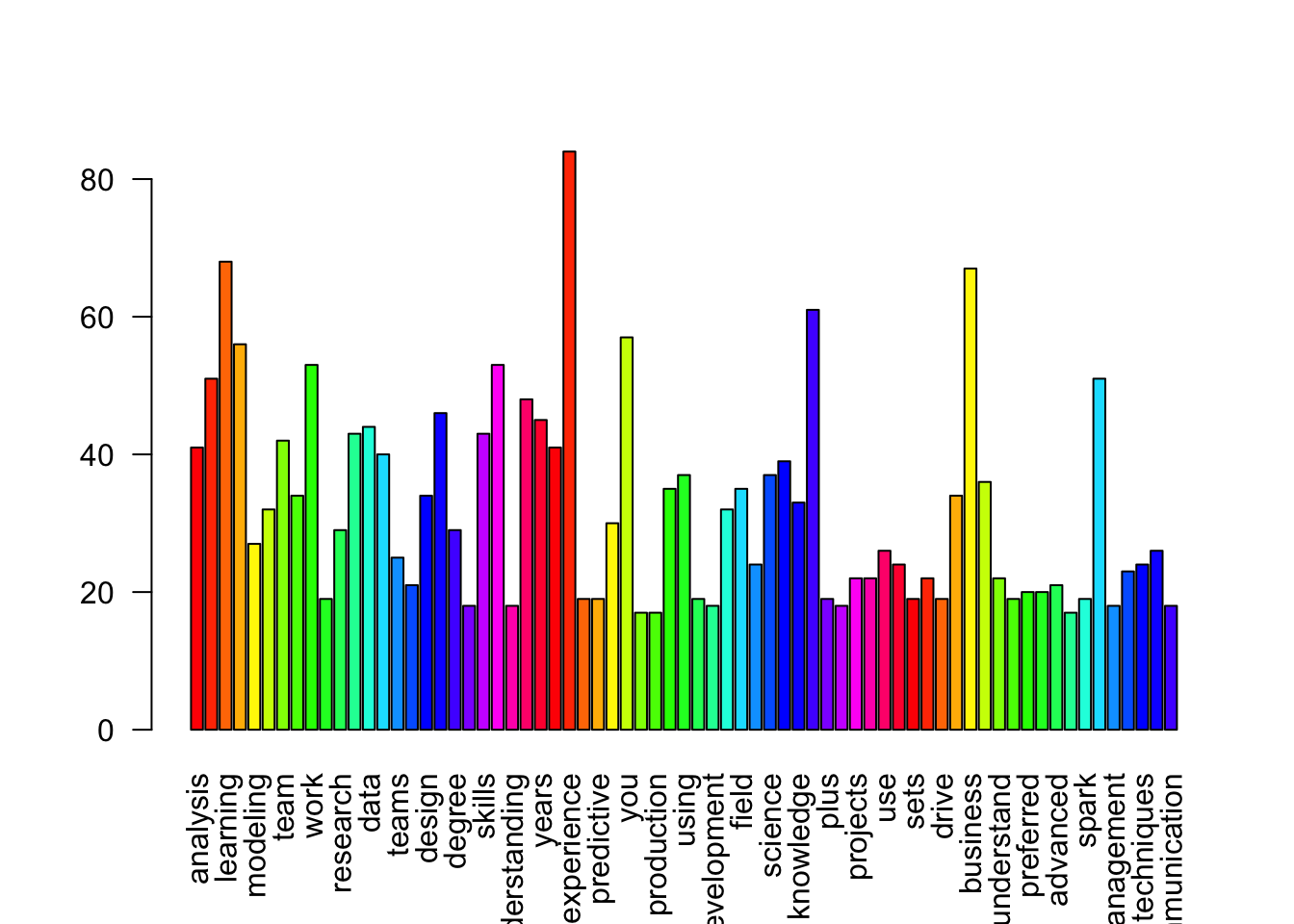

6. Generate world cloud

set.seed(1999) # for reproducibility
wordcloud(words = df$word,freq = df$frequency, min.freq = 20,
max.words = 80, random.order = F, rot.per = 0.25, scale = c(3, .3), colors = palette())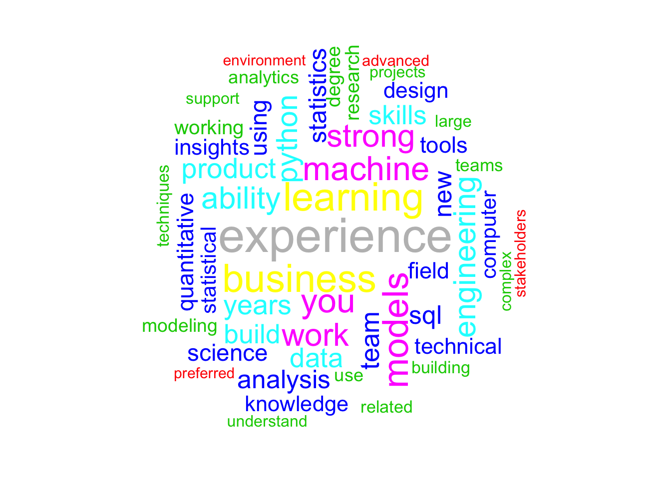

wordcloud2 package is a great alternative to create interactive word cloud.

set.seed(2000)
w <- data.frame(names(v), v)
colnames(w) <- c('word', 'freq')
wordcloud2(w,
           size = 0.30,
           shape = 'star',
           rotateRatio = 0.5,
           minSize = 1)

That’s how we build a word cloud. The most used keywords standout better in a word cloud. World clouds are easy to understand descriptive tool, visually engaging, simple yet impactful. However, analysis are limited to the insights of data. More extensive statistical analysis may be required for deep understanding of the data.

NLP