Topic Modeling on Gutenberg books
Topic modeling is an unsupervised machine learning technique for text data. It scans a set of documents(book chapters in this case), detecting word and phrase patterns within them, and clustering word groups and similar expressions that best characterize a set of documents.
Latent Dirichlet Allocation (LDA) is an example of topic modeling algorithm used to cluster text in a document to a particular topic. It is guided by two principles - every document is a mixture of topics and every topic is a mixture of words.
Suppose we have four books from Project Gutenberg library sub-categories: Crime, Music, Astronomy and Revolution. We tore the books into pages and shuffled without reading them.
Let’s use topic modeling using LDA algorithm to see whether it can correctly distinguish the four books.
Step-by-step explanations are as follows:
library(pacman)
p_load(topicmodels,gutenbergr,tidyverse,tidytext,stringr,scales)
1.Book Titles
# four books for topic models
titles <- c("Buccaneers and Pirates of Our Coasts", "Beethoven", "Astronomy for Amateurs","The Psychology of Revolution")
titles
## [1] "Buccaneers and Pirates of Our Coasts"
## [2] "Beethoven"
## [3] "Astronomy for Amateurs"
## [4] "The Psychology of Revolution"# retrieve books from gutenbergr
books <- gutenberg_download(c(448,15141,25267,17188), meta_fields = "title")2.Pre-Processing
# divide into documents, each representing one chapter
by_chapter <- books %>%
  group_by(title) %>%
  mutate(chapter = cumsum(str_detect(text, regex("^chapter ", ignore_case = TRUE)))) %>%
  ungroup() %>%
  filter(chapter > 0) %>%
  unite(document, title, chapter)

# split into words
by_chapter_word <- by_chapter %>%
  unnest_tokens(word, text)

# find document-word counts
word_counts <- by_chapter_word %>%
  anti_join(stop_words) %>%
  count(document, word, sort = TRUE) %>%
  ungroup()
## Joining, by = "word"word_counts## # A tibble: 67,284 x 3
## document word n
## <chr> <chr> <int>
## 1 "Beethoven, a character study\r\nTogether with Wagner's indeb… beethov… 87
## 2 "Astronomy for Amateurs_11" distance 77
## 3 "Astronomy for Amateurs_4" sun 66
## 4 "Astronomy for Amateurs_9" moon 64
## 5 "Astronomy for Amateurs_3" stars 63
## 6 "Astronomy for Amateurs_11" sun 58
## 7 "Astronomy for Amateurs_8" earth 56
## 8 "Astronomy for Amateurs_10" sun 54
## 9 "Astronomy for Amateurs_2" stars 53
## 10 "The Psychology of Revolution_53" revolut… 52
## # … with 67,274 more rows3.LDA on Chapters
# convert tidy data to document term matrix
chapters_dtm <- word_counts %>% cast_dtm(document, word, n)
chapters_dtm
## <<DocumentTermMatrix (documents: 117, terms: 16265)>>
## Non-/sparse entries: 67284/1835721
## Sparsity : 96%
## Maximal term length: 41
## Weighting : term frequency (tf)# create topic model with LDA function for four books, k = 4
chapters_lda <- LDA(chapters_dtm, k = 4, control = list(seed = 1999))
chapters_lda## A LDA_VEM topic model with 4 topics.#per-topic-per-word probabilities : beta
chapter_topics <- tidy(chapters_lda, matrix = "beta")
chapter_topics## # A tibble: 65,060 x 3
## topic term beta
## <int> <chr> <dbl>
## 1 1 beethoven 6.55e-135
## 2 2 beethoven 4.39e- 18
## 3 3 beethoven 1.34e-132
## 4 4 beethoven 2.09e- 2
## 5 1 distance 7.99e- 4
## 6 2 distance 9.49e- 5
## 7 3 distance 7.75e- 3
## 8 4 distance 7.62e- 5
## 9 1 sun 8.19e- 5
## 10 2 sun 3.16e- 5
## # … with 65,050 more rowsFor example, the term “beethoven” has zero probability of being generated from topics 1, 3, or 4, but it makes up 2% of topic 2.
# top 10 terms in each topic
top_terms <- chapter_topics %>% group_by(topic) %>%
  top_n(10, beta) %>% ungroup() %>%
  arrange(topic, -beta)
top_terms
## # A tibble: 40 x 3
## topic term beta
## <int> <chr> <dbl>
## 1 1 pirate 0.0117
## 2 1 pirates 0.0108
## 3 1 town 0.00865
## 4 1 vessel 0.00851
## 5 1 ship 0.00733
## 6 1 buccaneers 0.00622
## 7 1 time 0.00606
## 8 1 captain 0.00602
## 9 1 spanish 0.00585
## 10 1 people 0.00483
## # … with 30 more rows# visualize top terms from each topic
top_terms %>% mutate(term = reorder_within(term, beta, topic)) %>%
ggplot(aes(term, beta, fill = factor(topic))) +
geom_col(show.legend = F) + facet_wrap(~topic, scales = "free") +
coord_flip() + scale_x_reordered() +
labs(caption = "Fig:The terms that are most common within each topic") + theme(plot.caption = element_text(hjust = 0.5, size = 10))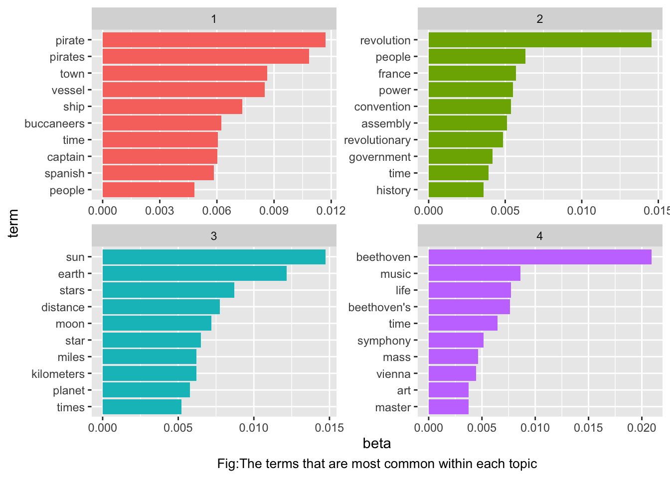
The topics are clearly associated with the four books.
4.Per-document Classification
#per-document-per-topic probabilities: gamma
chapters_gamma <- tidy(chapters_lda, matrix = "gamma")
chapters_gamma
## # A tibble: 468 x 3
## document topic gamma
## <chr> <int> <dbl>
## 1 "Beethoven, a character study\r\nTogether with Wagner's inde… 1 4.05e-6
## 2 "Astronomy for Amateurs_11" 1 7.54e-6
## 3 "Astronomy for Amateurs_4" 1 9.32e-6
## 4 "Astronomy for Amateurs_9" 1 1.05e-5
## 5 "Astronomy for Amateurs_3" 1 8.14e-6
## 6 "Astronomy for Amateurs_8" 1 8.58e-6
## 7 "Astronomy for Amateurs_10" 1 8.42e-6
## 8 "Astronomy for Amateurs_2" 1 9.93e-6
## 9 "The Psychology of Revolution_53" 1 7.75e-6
## 10 "Buccaneers and Pirates of Our Coasts_33" 1 1.00e+0
## # … with 458 more rowsAstronomy for Amateurs_11 document has 0% probability of coming from topic 1(Buccaneers and Pirates of Our Coasts).
#separate out chapter and title
chapters_gamma <- chapters_gamma %>%
  separate(document, c("title", "chapter"), sep= "_", convert = TRUE)
chapters_gamma
## # A tibble: 468 x 4
## title chapter topic gamma
## <chr> <int> <int> <dbl>
## 1 "Beethoven, a character study\r\nTogether with Wagne… 19 1 4.05e-6
## 2 "Astronomy for Amateurs" 11 1 7.54e-6
## 3 "Astronomy for Amateurs" 4 1 9.32e-6
## 4 "Astronomy for Amateurs" 9 1 1.05e-5
## 5 "Astronomy for Amateurs" 3 1 8.14e-6
## 6 "Astronomy for Amateurs" 8 1 8.58e-6
## 7 "Astronomy for Amateurs" 10 1 8.42e-6
## 8 "Astronomy for Amateurs" 2 1 9.93e-6
## 9 "The Psychology of Revolution" 53 1 7.75e-6
## 10 "Buccaneers and Pirates of Our Coasts" 33 1 1.00e+0
## # … with 458 more rows# reorder titles and plot
chapters_gamma %>% mutate(title = reorder(title, gamma*topic)) %>%
ggplot(aes(factor(topic),gamma)) + geom_boxplot() + facet_wrap(~title) +
labs(caption = "Fig: The gamma probabilities for each chapter within each book") + theme(plot.caption = element_text(hjust = 0.5, size = 12))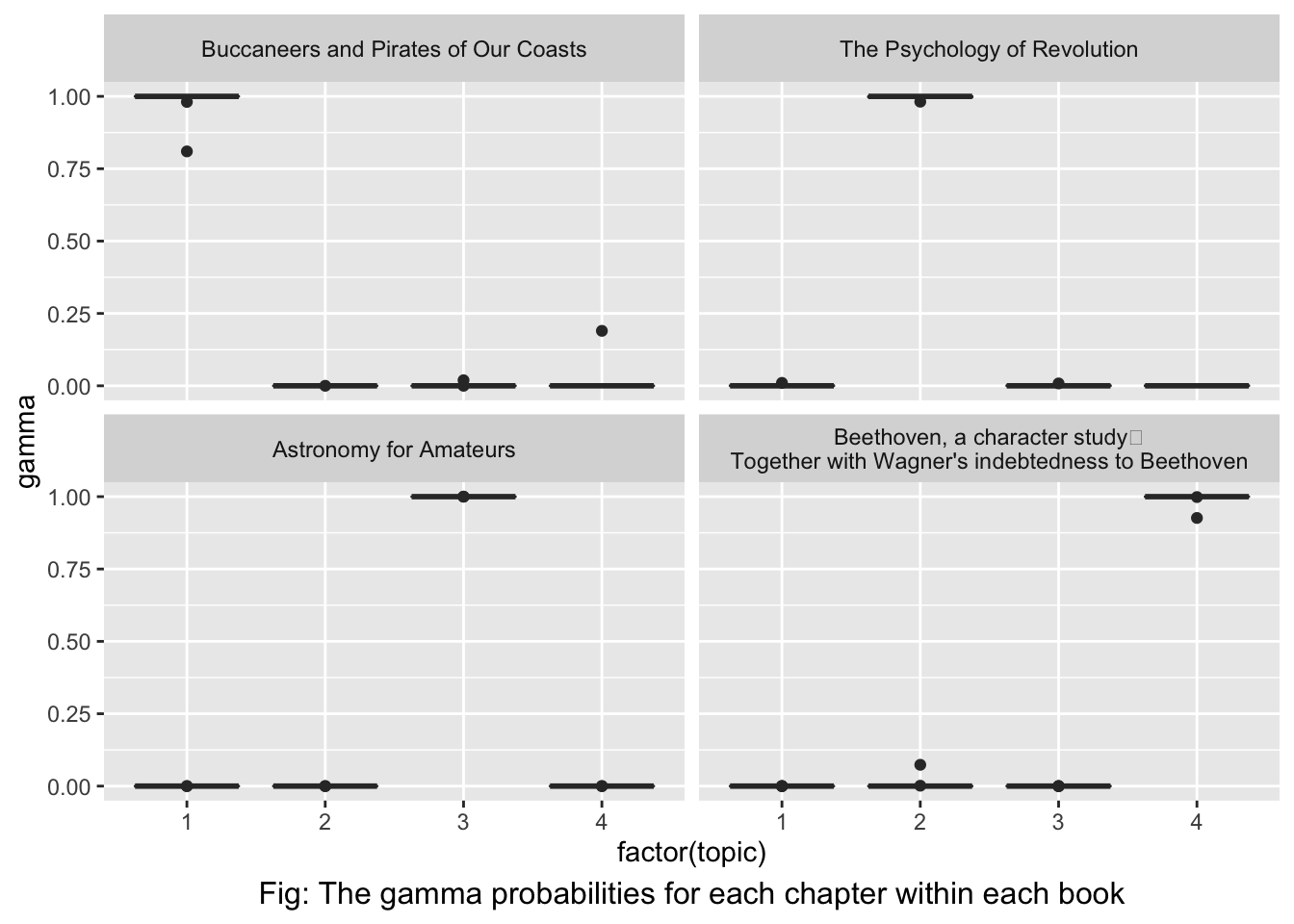
It appears all of the chapters are uniquely identified as a single topic.
#topic most associated with a chapter
chapter_classifications <- chapters_gamma %>%
  group_by(title, chapter) %>% top_n(1, gamma) %>%
  ungroup()
chapter_classifications
## # A tibble: 117 x 4
## title chapter topic gamma
## <chr> <int> <int> <dbl>
## 1 Buccaneers and Pirates of Our Coasts 33 1 1.00
## 2 Buccaneers and Pirates of Our Coasts 11 1 1.00
## 3 Buccaneers and Pirates of Our Coasts 31 1 1.00
## 4 Buccaneers and Pirates of Our Coasts 32 1 0.981
## 5 Buccaneers and Pirates of Our Coasts 30 1 1.00
## 6 Buccaneers and Pirates of Our Coasts 20 1 1.00
## 7 Buccaneers and Pirates of Our Coasts 21 1 1.00
## 8 Buccaneers and Pirates of Our Coasts 23 1 1.00
## 9 Buccaneers and Pirates of Our Coasts 15 1 1.00
## 10 Buccaneers and Pirates of Our Coasts 16 1 1.00
## # … with 107 more rows# consensus topics
book_topics <- chapter_classifications %>% count(title, topic) %>%
group_by(title) %>% top_n(1,n) %>% ungroup() %>%
transmute(consensus = title, topic)
book_topics%>% arrange((topic))## # A tibble: 4 x 2
## consensus topic
## <chr> <int>
## 1 "Buccaneers and Pirates of Our Coasts" 1
## 2 "The Psychology of Revolution" 2
## 3 "Astronomy for Amateurs" 3
## 4 "Beethoven, a character study\r\nTogether with Wagner's indebtedness to… 4#misidentified topics
chapter_classifications %>% inner_join(book_topics, by = "topic") %>%
filter(title != consensus)## # A tibble: 0 x 5
## # … with 5 variables: title <chr>, chapter <int>, topic <int>, gamma <dbl>,
## # consensus <chr>Indeed, no chapters were mis-classified.
5.By Word Assignments: Augment
# see which words are assigned to which topic with augment function
assignments <- augment(chapters_lda, data = chapters_dtm)
assignments
## # A tibble: 67,284 x 4
## document term count .topic
## <chr> <chr> <dbl> <dbl>
## 1 "Beethoven, a character study\r\nTogether with Wagner's… beetho… 87 4
## 2 "Beethoven, a character study\r\nTogether with Wagner's… beetho… 45 4
## 3 "Beethoven, a character study\r\nTogether with Wagner's… beetho… 44 4
## 4 "Beethoven, a character study\r\nTogether with Wagner's… beetho… 43 4
## 5 "Beethoven, a character study\r\nTogether with Wagner's… beetho… 43 4
## 6 "Beethoven, a character study\r\nTogether with Wagner's… beetho… 39 4
## 7 "Beethoven, a character study\r\nTogether with Wagner's… beetho… 38 4
## 8 "Beethoven, a character study\r\nTogether with Wagner's… beetho… 28 4
## 9 "Beethoven, a character study\r\nTogether with Wagner's… beetho… 25 4
## 10 "Beethoven, a character study\r\nTogether with Wagner's… beetho… 24 4
## # … with 67,274 more rows# combine assignments with true book titles to find incorrect classification
assignments <- assignments %>%
separate(document, c("title", "chapter"), sep = "_", convert = TRUE)%>%
inner_join(book_topics, by = c(".topic" = "topic"))
assignments## # A tibble: 67,284 x 6
## title chapter term count .topic consensus
## <chr> <int> <chr> <dbl> <dbl> <chr>
## 1 "Beethoven, a characte… 19 beeth… 87 4 "Beethoven, a character …
## 2 "Beethoven, a characte… 13 beeth… 45 4 "Beethoven, a character …
## 3 "Beethoven, a characte… 8 beeth… 44 4 "Beethoven, a character …
## 4 "Beethoven, a characte… 1 beeth… 43 4 "Beethoven, a character …
## 5 "Beethoven, a characte… 6 beeth… 43 4 "Beethoven, a character …
## 6 "Beethoven, a characte… 2 beeth… 39 4 "Beethoven, a character …
## 7 "Beethoven, a characte… 10 beeth… 38 4 "Beethoven, a character …
## 8 "Beethoven, a characte… 5 beeth… 28 4 "Beethoven, a character …
## 9 "Beethoven, a characte… 11 beeth… 25 4 "Beethoven, a character …
## 10 "Beethoven, a characte… 14 beeth… 24 4 "Beethoven, a character …
## # … with 67,274 more rows#visualize a confusion matrix
assignments %>%
count(title, consensus, wt = count) %>%
group_by(title) %>%
mutate(percent = n / sum(n)) %>%
ggplot(aes(consensus, title, fill = percent)) +
geom_tile() +
scale_fill_gradient2(high = "blue", label = percent_format()) +
theme_minimal() +
theme(axis.text.x = element_text(angle = 90, hjust = 1),
panel.grid = element_blank()) +
labs(x = "book words were assigned to",
y = "book words came from",
fill = "% of assignments") +
labs(caption = "Fig: Confusion matrix showing where LDA assigned the words from each book") +
theme(plot.caption = element_text( size = 10),legend.key.size = unit(0.5, "cm")) 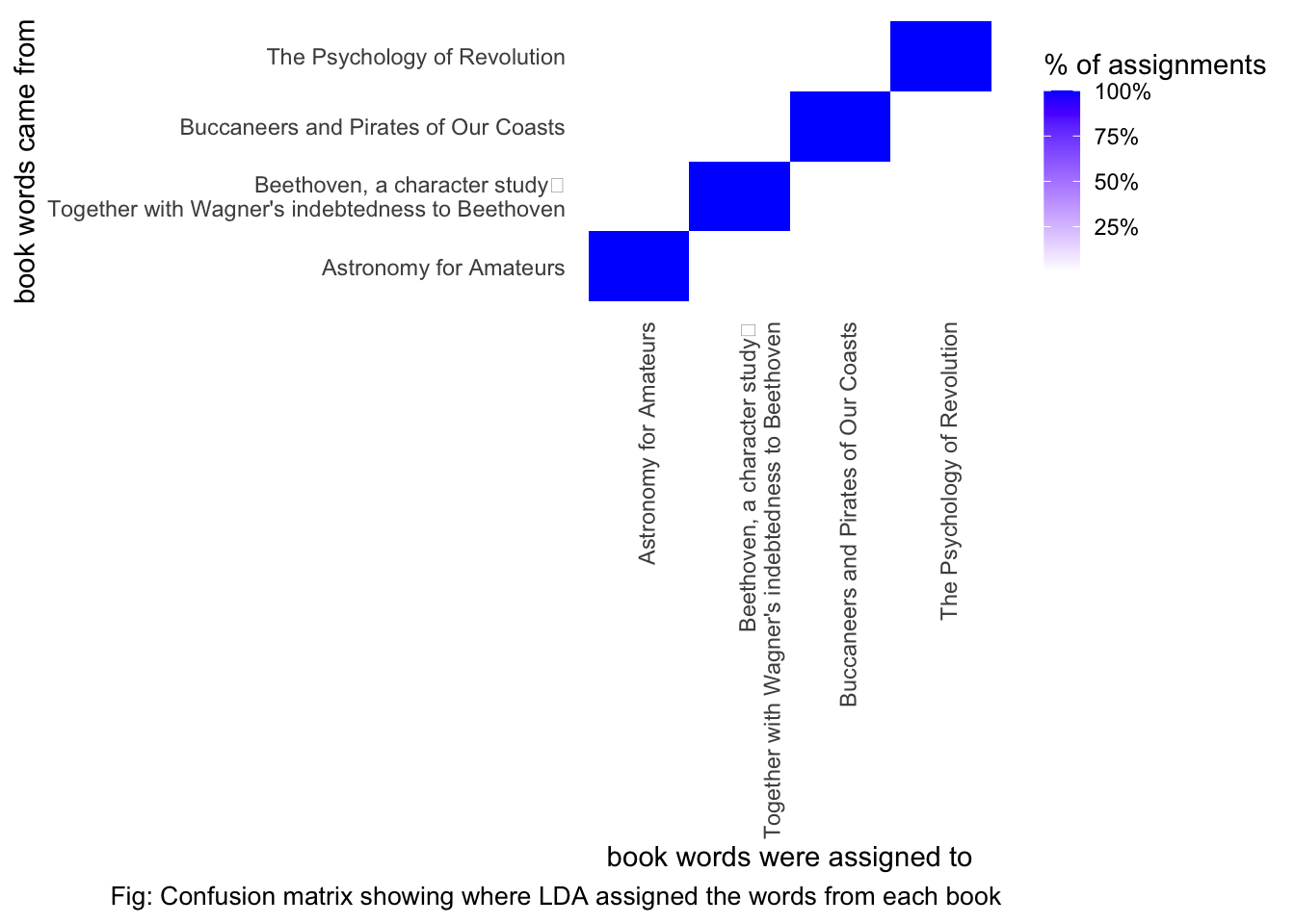
Almost all words were correctly assigned to each topic.
# most commonly mistaken words
wrong_words <- assignments %>% filter(title!= consensus)
wrong_words
## # A tibble: 45 x 6
## title chapter term count .topic consensus
## <chr> <int> <chr> <dbl> <dbl> <chr>
## 1 "Buccaneers and Pirate… 32 moon 3 3 "Astronomy for Amateurs"
## 2 "Buccaneers and Pirate… 32 stars 2 3 "Astronomy for Amateurs"
## 3 "Beethoven, a characte… 4 revol… 1 2 "The Psychology of Revol…
## 4 "The Psychology of Rev… 45 capta… 1 1 "Buccaneers and Pirates …
## 5 "The Psychology of Rev… 45 town 2 1 "Buccaneers and Pirates …
## 6 "Buccaneers and Pirate… 32 heave… 1 3 "Astronomy for Amateurs"
## 7 "The Psychology of Rev… 45 vessel 1 1 "Buccaneers and Pirates …
## 8 "Beethoven, a characte… 4 armies 2 2 "The Psychology of Revol…
## 9 "Buccaneers and Pirate… 1 1 1 4 "Beethoven, a character …
## 10 "Beethoven, a characte… 4 bonap… 3 2 "The Psychology of Revol…
## # … with 35 more rowswrong_words %>% count(title, consensus, term , wt = count) %>%
ungroup() %>% arrange(-n)## # A tibble: 45 x 4
## title consensus term n
## <chr> <chr> <chr> <dbl>
## 1 "Beethoven, a character study\r\nTogeth… The Psychology of Revo… france 6
## 2 "Beethoven, a character study\r\nTogeth… The Psychology of Revo… bonap… 3
## 3 "Buccaneers and Pirates of Our Coasts" Astronomy for Amateurs moon 3
## 4 "Beethoven, a character study\r\nTogeth… The Psychology of Revo… armies 2
## 5 "Beethoven, a character study\r\nTogeth… The Psychology of Revo… louis 2
## 6 "Buccaneers and Pirates of Our Coasts" Astronomy for Amateurs stars 2
## 7 "The Psychology of Revolution" Buccaneers and Pirates… town 2
## 8 "Beethoven, a character study\r\nTogeth… The Psychology of Revo… equal… 1
## 9 "Beethoven, a character study\r\nTogeth… The Psychology of Revo… gover… 1
## 10 "Beethoven, a character study\r\nTogeth… The Psychology of Revo… illus… 1
## # … with 35 more rowsThe word “moon” and “stars” appear in “Buccaneers and Pirates of Our Coasts” but they are wrongly classified into “Astronomy for Amateurs” becuase they are more common in the later.
# wrongly classified word, eg. "moon"
word_counts %>% filter(word == "moon")
## # A tibble: 12 x 3
## document word n
## <chr> <chr> <int>
## 1 Astronomy for Amateurs_9 moon 64
## 2 Astronomy for Amateurs_10 moon 49
## 3 Astronomy for Amateurs_11 moon 35
## 4 Astronomy for Amateurs_4 moon 10
## 5 Astronomy for Amateurs_12 moon 9
## 6 Astronomy for Amateurs_5 moon 8
## 7 Astronomy for Amateurs_8 moon 4
## 8 Astronomy for Amateurs_3 moon 3
## 9 Astronomy for Amateurs_6 moon 3
## 10 Buccaneers and Pirates of Our Coasts_32 moon 3
## 11 Astronomy for Amateurs_1 moon 2
## 12 Astronomy for Amateurs_7 moon 2Although the words are presumably different for each topic since books are selected from different genre, LDA algorithm performed really well on identifying topics to the document and words to the topic. Really great for unsupervised clustering!